
Machine Learning is most widely done using Python and scikit-learn toolkit. The biggest disadvantage of using this combination is the single machine limit that Python imposes on training the model. This limits the amount of data that can be used for training to the maximum memory on the computer.

Industrial/ enterprise datasets tend to be in terabytes and hence the need for a parallel processing framework that could handle enormous datasets was felt. This is where Spark comes in. Spark comes with a machine learning framework that can be executed in parallel during training using a framework called Spark ML. Spark ML is based on the same Dataframe API that is widely used within the Spark ecosystem. This requires minimal additional learning for preprocessing of raw data.
In this post, we will cover how to train a model using Spark ML.
In the next post, we will introduce the concept of Spark ML pipelines that allow us to process the data in a defined sequence.
The final post will cover MLOps capabilities that MLFlow framework provides for operationalising our machine learning models.
We are going to be Adult Dataset from UCI Machine Learning Repository. Go ahead and download the dataset from the “Data Folder” link on the page. The file you are interested to download is named “adult.data” and contains the actual data. Since the format of this dataset is CSV, I saved it on my local machine as adult.data.csv. The schema of this dataset is available in another file titled – adult.names. The schema of the dataset is as follows:
age: continuous.
workclass: categorical.
fnlwgt: continuous.
education: categorical.
education-num: continuous.
marital-status: categorical.
race: categorical.
sex: categorical.
capital-gain: continuous.
capital-loss: continuous.
hours-per-week: continuous.
native-country: categorical.
summary: categorical
The prediction task is to determine whether a person makes over 50K in a year which is contained in the summary field. This field contains value of <50K or >=50K and is our target variable. The machine learning task is that of binary classification.

The first step was to upload the dataset from where it is accessible. I chose DBFS for ease of use and uploaded the file at the following location: /dbfs/FileStore/Abhishek-kant/adult_dataset.csv
Once loaded in DBFS, we need to access the same as a Dataframe. We will apply a schema while reading the data since the data doesn’t come with header values as indicated below:
adultSchema = "age int,workclass string,fnlwgt float,education string,educationnum float,maritalstatus string,occupation string,relationship string,race string,sex string,capitalgain double,capitalloss double,hoursperweek double,nativecountry string,category string"

adultDF = spark.read.csv("/FileStore/Abhishek-kant/adult_dataset.csv", inferSchema = True, header = False, schema = adultSchema)
A sample of the data is shown below:
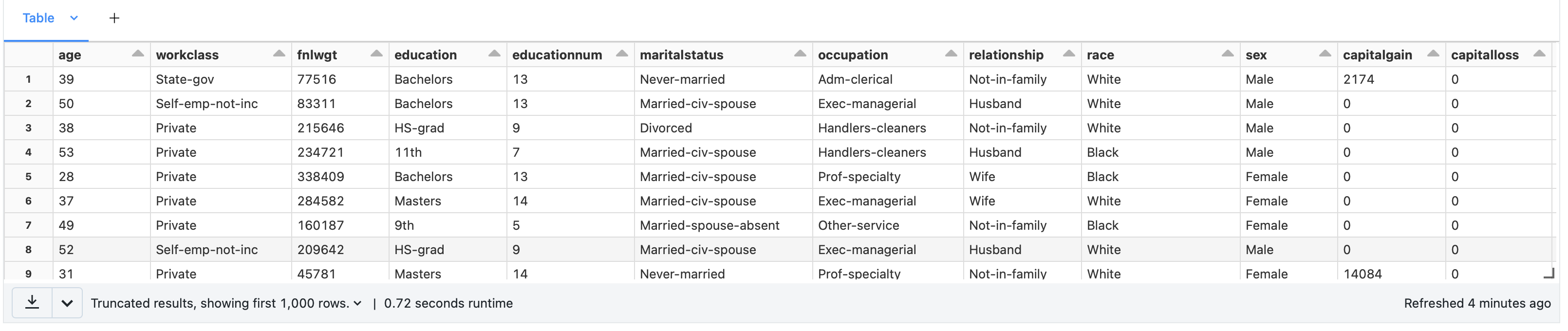
We need to move towards making this dataset machine learning ready. Spark ML only works with numeric data. We have many text values in the dataframe that will need to be converted to numeric values.
One of the key changes is to convert categorical variables expressed as string into labels expressed as string. This can be done using StringIndexer object (available in pyspark.ml.feature namespace) as illustrated below:
eduindexer = StringIndexer(inputCol=”education”, outputCol =”edu”)
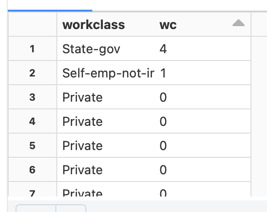
The inputCol indicates the column to be transformed and outputCol is the name of the column that will get added to the dataframe after converting to the categorical label. The result of the StringIndexer is shown to the right e.g. Private is converted to 0 while State-gov is converted to 4.
This conversion will need to be done for every column:
#Convert Categorical variables to numeric
from pyspark.ml.feature import StringIndexer

wcindexer = StringIndexer(inputCol="workclass", outputCol ="wc")
eduindexer = StringIndexer(inputCol="education", outputCol ="edu")
maritalindexer = StringIndexer(inputCol="maritalstatus", outputCol ="marital")
occupationindexer = StringIndexer(inputCol="occupation", outputCol ="occ")
relindexer = StringIndexer(inputCol="relationship", outputCol ="relation")
raceindexer = StringIndexer(inputCol="race", outputCol ="racecolor")
sexindexer = StringIndexer(inputCol="sex", outputCol ="gender")
nativecountryindexer = StringIndexer(inputCol="nativecountry", outputCol ="country")
categoryindexer = StringIndexer(inputCol="category", outputCol ="catlabel")
This creates what is called a “dense” matrix where a single column contains all the values. Further, we will need to convert this to “sparse” matrix where we have multiple columns for each value for a category and for each column we have a 0 or 1. This conversion can be done using the OneHotEncoder object (available in pyspark.ml.feature namespace) as shown below:
ohencoder = OneHotEncoder(inputCols=[“wc”], outputCols=[“v_wc”])

The inputCols is a list of columns that need to be “sparsed” and outputCols is the new column name. The confusion sometimes is around fitting sparse matrix in a single column. OneHotEncoder uses a schema based approach to fit this in a single column as shown to the left.
Note that we will not sparse the target variable i.e. “summary”.
The final step for preparing our data for machine learning is to “vectorise” it. Unlike most machine learning frameworks that take a matrix for training, Spark ML requires all feature columns to be passed in as a single vector of columns. This is achieved using VectorAssembler object (available in pyspark.ml.feature namespace) as shown below:
colvectors = VectorAssembler(inputCols=["age","v_wc","fnlwgt","educationnum","capitalgain","capitalloss","v_edu","v_marital","v_occ","v_relation","v_racecolor","v_gender","v_country","hoursperweek"],
outputCol="features")
As you can see above, we are adding all columns in a vector called as “features”. With this our dataframe is ready for machine learning task.
We will proceed to split the dataframe in training and test data set using randomSplit function of dataframe as shown:
(train, test) = adultMLDF.randomSplit([0.7,0.3])
This will split our dataframe into train and test dataframe in 70:30 ratio.
The classifier used will be Gradient Boosting classifier available as GBTClassifier object and initialised as follows:
from pyspark.ml.classification import GBTClassifier

classifier = GBTClassifier(labelCol="catlabel", featuresCol="features")
The target variable and features vector column is passed as attributes to the object. Once the classifier object is initialised we can use it to train our model using the “fit” method and passing the training dataset as an attribute:
gbmodel = classifier.fit(train)
Once the training is done, you can get predictions on the test dataset using the “transform” method of the model with test dataset passed in as attribute:
adultTestDF = gbmodel.transform(test)
The result of this function is addition of three columns to the dataset as shown below:

A very important task in machine learning is to determine the efficacy of the model. To evaluate how the model performed, we can use the BinaryClassificationEvaluator object as follows:
from pyspark.ml.evaluation import BinaryClassificationEvaluator

eval = BinaryClassificationEvaluator(labelCol = "catlabel", rawPredictionCol="rawPrediction")

eval.evaluate(adultTestDF)
In the initialisation of the BinaryClassificationEvaluator, the labelCol attribute specifies the actual value and rawPredictionCol represents the predicted value stored in the column – rawPrediction. The evaluate function will give the accuracy of the prediction in the test dataset represented as AreaUnderROC metric for classification tasks.
You would definitely want to save the trained model for use later by simply saving the model as follows:
gbmodel.save(path)
You can later retrieve this model using “load” function of the specific classifier:
from pyspark.ml.classification import GBTClassificationModel
classifierModel = GBTClassificationModel.load(path)
You can now use this classification model for inferencing as required.

Pingback: Introduction to Machine Learning with Spark ML – II | Telerik Helper - Helping Ninja Technologists