Introduction to Machine Learning with Spark ML – III

In the last post, we saw how we can use Pipelines to streamline our machine learning workflow.

We will start off with a fantastic feature that will blow the lid off your mind. All the effort done till now, in post I and II, can be done in 2 lines of code! Ah yes, this magic is possible with use of a feature called AutoML. Not only will it perform preprocessing steps automatically, it will also select the best algorithm from a multitude of them including XGBoost, LightGBM, Prophet etc. The hyper parameter search comes for free 🙂 If all this was not enough it will share the entire auto-generated code for your use and modification. So, the two magic lines are:

from databricks import automl
summary = automl.classify(train, target_col="category", timeout_minutes=20)

The AutoML requires you to specify the following:

  1. Type of machine learning problem – Classification/ Regression/ Forecasting
  2. Specify the training set, target column
  3. Timeout after which the autoML will stop looking for better models.

While all this is very exciting, the real world use case of AutoML tends to be to create a baseline for model performance and give us a model to start with. In our case, the AutoML gave an RoC score of 91.8% (actually better than our manual work so far!!) for the best model.

Looking at the auto-generated Python notebook, here are the broad steps it took:

  1. Load Data
  2. Preprocessing
    • Impute values for missing numerical columns
    • Convert each categorical column into multiple binary columns through one-hot encoding
  3. Train – Validation – Test Split
  4. Train classification model
  5. Inference
  6. Determine Accuracy – Confusion matrix, ROC and Precision-Recall curves for validation data

This is broadly in line with what we did in our manual setup.

Apart from the coded approach we saw, you can create AutoML experiment using the UI from the Experiments -> Create AutoML Experiment button. If you can’t find the experiments tab, make sure that you have the Machine Learning persona selected in the Databricks workspace.

In an enterprise/ real world scenario, we will build many alternate models with different parameters and use the one with higest accuracy. Next, we deploy the model and use it for predictions with new data. Finally, the selected model will be updated over time as new data becomes available. Until now, we didn’t talk about how to handle these enterprise requirements or were doing it manually on best effort.

These requirements are covered under what we know as MLOps. Spark supports MLOps using an open source framework called MLFlow. MLFlow supports the following objects:

  1. Projects: Provides a mechanism for storing machine learning code in a reusable and reproducible format.
  2. Tracking: Allows for tracking your experiments and metrics. You can see the history of your model and its accuracy evolve over time. There is also a tracking UI available.
  3. Model Registry: Allows for storing various models that you develop in a registry with an UI to explore the same. It also provides for model lineage (which MLflow experiment and run produced the model), stage transitions (for example from staging to production)
  4. Model Serving: We can use serving to provide inference endpoints for either batch or inline processing. Mostly this will be made available as REST endopoints.

There is a very easy way to get started with MLFlow where we allow MLFlow to log automatically the metrics and models. This can be done using a single line:

import mlflow
mlflow.autolog()

This will log the parameters, metrics, models and the environment. The core concept to get with MLOps is the concept of runs. Each run is a unique combination of parameters and algorithm that you have executed. Many runs can be part of the same experiment.

To get started we can set name of the experiment with the command: mlflow_set_experiment(“name_of_the_experiment”)

To start tracking the experiments manually, we can setup the context as follows:

with mlflow.start_run(run_name="") as run:
   <pseudo code for running an experiment>
   mlflow.log_param("key","value")
   mlflow.log_metrics("key","value")
   mlflow.spark.log_model(model,"model name")

You can track parameters and metrics using log_param and log_metrics functions of mlflow object. The model can now be registered with the Model Registry using the function: mlflow.register_model(model_uri=””, name=””)

What is important here is the model_uri. The model_uri takes the form: runs:/<runid>/model. The runid identifies the specific run in the experiment and each model is stored at the model_uri location mentioned above.

You can now load the model and perform inference using the following code:

import mlflow

# Load model
loaded_model = mlflow.spark.load_model(model_uri)

# Perform inference via model.transform()
loaded_model.transform(data)

While we have seen how to track experiments explicitly, Databricks Workspaces also track the experiments automatically (from Databricks Runtime 10.3 ML and above). You can view the expriments and their runs in the UI via the Experiments sidebar of the Machine Learning persona.

You will need to click on the specific experiment (in our case Adult Dataset), that will show all the runs of the experiment. Click on the specific run to get more details about the run. The run will show the metrics recorded which is in our case was areaUnderRoC of 91.4%.

Under Artifacts, if you click on the model, you can see the URI of the model run. This URI can be used to register the model with the Model Registry and use it for predictions at any point in time.

MLFlow also supports indicating the state of the model for production. Different states supported by MLFlow are:

  1. None
  2. Staging
  3. Production
  4. Archived

Once your model is registered with the Model registry, you can change the state of the model to any other state with the function transition_model_version_stage() function.

From the model registry you are able to create model serving endpoint using the Serverless Real-Time Inference service that uses managed Databricks compute service to provide a REST endpoint.

Advertisement

Introduction to Machine Learning with Spark ML – II

In the earlier post, we went over some concepts regarding Machine Learning done with Spark ML. Here are primarily 2 types of objects relating to machine learning we saw:

  1. Transformers: Objects that took a DataFrame, changed something in it and returned a DataFrame. The method used here was “transform”.
  2. Estimator: Objects that are passed in a DataFrame and would apply an algorithm on it to return a transformer. E.g. GBTClassifier. We used the “fit” function to apply the algorithm on the Dataframe.

In our last example of predicting income level using Adult dataset, we had to change our input dataset to a format that is suitable for machine learning. There was a sequence of changes we had done e.g. converting categorical variables to numeric, One Hot Encoding & Assembling the columns in a single column. Everytime there is additional data available (which will be numerous times), we will need to do these steps again and again.

In this post, we will introduce a new Object that organises these steps in sequence that can be run as many times as needed and it is called the Pipeline. The Pipeline chains together various transformers and estimators in sequence. While we could do the machine learning without the Pipeline, it is a standard practice to put the sequence of steps in a Pipeline. Before we get there, let’s try to add an additional step in fixing our pipeline and that is to identify and remove Null data. This is indicated in our dataset as ‘?’.

To know how many null values exist let’s run this command:

from pyspark.sql.functions import isnull, when, count, col
adultDF.select([count(when(isnull(c), c)).alias(c) for c in adultDF.columns]).show()

The result shows that there are no null values. Inspecting the data, we see that null values have been replaced with “?”. We would need to remove these rows from our dataset. We can replace the ? with null values as follows:

adultDF = adultDF.replace('?', None)

Surprisingly this doesn’t change the ? values. It appeared that the ? is padded with some spaces. So we will use the when and trim function as follows:

from pyspark.sql.functions import isnull, when, count, col,trim
adultDF = adultDF.select([when(trim(col(c))=='?',None).otherwise(col(c)).alias(c) for c in adultDF.columns])

This replaces ? will null that we can now drop from our dataframe using dropna() function. The number of rows remaining are now 30,162.

Now let’s organise these steps in a Pipeline as follows:

from pyspark.ml import Pipeline

adultPipeline = Pipeline(stages = [wcindexer,eduindexer,maritalindexer,occupationindexer,relindexer,raceindexer,sexindexer,nativecountryindexer,categoryindexer,ohencoder,colvectors])

The stages list contains all the transformers we used to convert raw data into dataset ready for machine learning. This includes all the StringIndexers, OneHotEncoder and VectorAssembler. Next, the process of defining the GBTClassifier and BinaryClassificationEvaluator remains the same as in the earlier post. You can now include the GBTClassfier in the pipeline as well and run the fit() on this pipeline with train dataset as follows:

adultMLTrainingPipeline = Pipeline(stages = [adultPipeline,gbtclassifier])
gbmodel  = adultMLTrainingPipeline.fit(train)

However, we can perform another optimization at this point. The model currently trained is based of a random split of values from the dataset. Cross Validation can help generalise the model even better by determining best parameters from a list of parameters and do it by creating more than one train and test datasets (called as folds). The list of parameters are supplied as ParamGrid as follows:

from pyspark.ml.tuning import CrossValidator, ParamGridBuilder

paramGrid = ParamGridBuilder()\
  .addGrid(gbtclassifier.maxDepth, [2, 5])\
  .addGrid(gbtclassifier.maxIter, [10, 100])\
  .build()

# Declare the CrossValidator, which performs the model tuning.
cv = CrossValidator(estimator=gbtclassifier, evaluator=eval, estimatorParamMaps=paramGrid)

The cross validator object takes the estimator, evaluator and the paramGrid objects. The pipeline will need to be modified to use this cross validator instead of the classifier object we used earlier as follows:

adultMLTrainingPipeline = Pipeline(stages = [adultPipeline,gbtclassifier])


adultMLTrainingPipeline = Pipeline(stages = [adultPipeline,cv])

With these settings, the experiment ran for 22 mins and the evalution result came out to be 91.37% area under RoC.

Introduction to Machine Learning with Spark ML – I

Machine Learning is most widely done using Python and scikit-learn toolkit. The biggest disadvantage of using this combination is the single machine limit that Python imposes on training the model. This limits the amount of data that can be used for training to the maximum memory on the computer.

Industrial/ enterprise datasets tend to be in terabytes and hence the need for a parallel processing framework that could handle enormous datasets was felt. This is where Spark comes in. Spark comes with a machine learning framework that can be executed in parallel during training using a framework called Spark ML. Spark ML is based on the same Dataframe API that is widely used within the Spark ecosystem. This requires minimal additional learning for preprocessing of raw data.

In this post, we will cover how to train a model using Spark ML.

In the next post, we will introduce the concept of Spark ML pipelines that allow us to process the data in a defined sequence.

The final post will cover MLOps capabilities that MLFlow framework provides for operationalising our machine learning models.

We are going to be Adult Dataset from UCI Machine Learning Repository. Go ahead and download the dataset from the “Data Folder” link on the page. The file you are interested to download is named “adult.data” and contains the actual data. Since the format of this dataset is CSV, I saved it on my local machine as adult.data.csv. The schema of this dataset is available in another file titled – adult.names. The schema of the dataset is as follows:

age: continuous.
workclass: categorical.
fnlwgt: continuous.
education: categorical.
education-num: continuous.
marital-status: categorical.
race: categorical.
sex: categorical.
capital-gain: continuous.
capital-loss: continuous.
hours-per-week: continuous.
native-country: categorical.
summary: categorical

The prediction task is to determine whether a person makes over 50K in a year which is contained in the summary field. This field contains value of <50K or >=50K and is our target variable. The machine learning task is that of binary classification.

Upload file in DBFS

The first step was to upload the dataset from where it is accessible. I chose DBFS for ease of use and uploaded the file at the following location: /dbfs/FileStore/Abhishek-kant/adult_dataset.csv

Once loaded in DBFS, we need to access the same as a Dataframe. We will apply a schema while reading the data since the data doesn’t come with header values as indicated below:

adultSchema = "age int,workclass string,fnlwgt float,education string,educationnum float,maritalstatus string,occupation string,relationship string,race string,sex string,capitalgain double,capitalloss double,hoursperweek double,nativecountry string,category string"

adultDF = spark.read.csv("/FileStore/Abhishek-kant/adult_dataset.csv", inferSchema = True, header = False, schema = adultSchema)

A sample of the data is shown below:

We need to move towards making this dataset machine learning ready. Spark ML only works with numeric data. We have many text values in the dataframe that will need to be converted to numeric values.

One of the key changes is to convert categorical variables expressed as string into labels expressed as string. This can be done using StringIndexer object (available in pyspark.ml.feature namespace) as illustrated below:
eduindexer = StringIndexer(inputCol=”education”, outputCol =”edu”)

The inputCol indicates the column to be transformed and outputCol is the name of the column that will get added to the dataframe after converting to the categorical label. The result of the StringIndexer is shown to the right e.g. Private is converted to 0 while State-gov is converted to 4.

This conversion will need to be done for every column:

#Convert Categorical variables to numeric
from pyspark.ml.feature import StringIndexer

wcindexer = StringIndexer(inputCol="workclass", outputCol ="wc")
eduindexer = StringIndexer(inputCol="education", outputCol ="edu")
maritalindexer = StringIndexer(inputCol="maritalstatus", outputCol ="marital")
occupationindexer = StringIndexer(inputCol="occupation", outputCol ="occ")
relindexer = StringIndexer(inputCol="relationship", outputCol ="relation")
raceindexer = StringIndexer(inputCol="race", outputCol ="racecolor")
sexindexer = StringIndexer(inputCol="sex", outputCol ="gender")
nativecountryindexer = StringIndexer(inputCol="nativecountry", outputCol ="country")
categoryindexer = StringIndexer(inputCol="category", outputCol ="catlabel")

This creates what is called a “dense” matrix where a single column contains all the values. Further, we will need to convert this to “sparse” matrix where we have multiple columns for each value for a category and for each column we have a 0 or 1. This conversion can be done using the OneHotEncoder object (available in pyspark.ml.feature namespace) as shown below:
ohencoder = OneHotEncoder(inputCols=[“wc”], outputCols=[“v_wc”])

The inputCols is a list of columns that need to be “sparsed” and outputCols is the new column name. The confusion sometimes is around fitting sparse matrix in a single column. OneHotEncoder uses a schema based approach to fit this in a single column as shown to the left.

Note that we will not sparse the target variable i.e. “summary”.

The final step for preparing our data for machine learning is to “vectorise” it. Unlike most machine learning frameworks that take a matrix for training, Spark ML requires all feature columns to be passed in as a single vector of columns. This is achieved using VectorAssembler object (available in pyspark.ml.feature namespace) as shown below:

colvectors = VectorAssembler(inputCols=["age","v_wc","fnlwgt","educationnum","capitalgain","capitalloss","v_edu","v_marital","v_occ","v_relation","v_racecolor","v_gender","v_country","hoursperweek"],
outputCol="features")

As you can see above, we are adding all columns in a vector called as “features”. With this our dataframe is ready for machine learning task.

We will proceed to split the dataframe in training and test data set using randomSplit function of dataframe as shown:

(train, test) = adultMLDF.randomSplit([0.7,0.3])

This will split our dataframe into train and test dataframe in 70:30 ratio.
The classifier used will be Gradient Boosting classifier available as GBTClassifier object and initialised as follows:

from pyspark.ml.classification import GBTClassifier

classifier = GBTClassifier(labelCol="catlabel", featuresCol="features")

The target variable and features vector column is passed as attributes to the object. Once the classifier object is initialised we can use it to train our model using the “fit” method and passing the training dataset as an attribute:

gbmodel = classifier.fit(train)

Once the training is done, you can get predictions on the test dataset using the “transform” method of the model with test dataset passed in as attribute:

adultTestDF = gbmodel.transform(test)

The result of this function is addition of three columns to the dataset as shown below:

A very important task in machine learning is to determine the efficacy of the model. To evaluate how the model performed, we can use the BinaryClassificationEvaluator object as follows:

from pyspark.ml.evaluation import BinaryClassificationEvaluator

eval = BinaryClassificationEvaluator(labelCol = "catlabel", rawPredictionCol="rawPrediction")

eval.evaluate(adultTestDF)

In the initialisation of the BinaryClassificationEvaluator, the labelCol attribute specifies the actual value and rawPredictionCol represents the predicted value stored in the column – rawPrediction. The evaluate function will give the accuracy of the prediction in the test dataset represented as AreaUnderROC metric for classification tasks.

You would definitely want to save the trained model for use later by simply saving the model as follows:

gbmodel.save(path)

You can later retrieve this model using “load” function of the specific classifier:

from pyspark.ml.classification import GBTClassificationModel
classifierModel = GBTClassificationModel.load(path)

You can now use this classification model for inferencing as required.

Azure Databricks – What is it costing me?

A customer wanted to know the total cost of running Azure Databricks for them. They couldn’t understand what DBU (Databricks Units) was, given that is the pricing unit for Azure Databricks.

I will attempt to clarify DBU in this post.

DBU is just really an abstraction not related to any amount of compute or compute metrics. At the same time, it changes with the following factors:

  1. When there is a change in the kind of machine you are running the cluster on
  2. When there is change in the kind of workload (e.g. Jobs, All Purpose)
  3. The tier / capabilities of the workload (Standard / Premium)
  4. The kind of runtime (e.g. with or without Photon)

So, the DBUs really measure the consumption of resources. It is billed on a per second basis. The monetary value of these DBUs is called $DBU and is determined by a $ rate charged per DBU. Pricing rate per DBU is available here.

You are paying DBUs for the software that Databricks has made available for processing your Big Data workload. The hardware component needed to run the cluster is charged directly by Azure.

When you visit the Azure Pricing Calculator and look at the pricing for Azure Databricks, you would see that there are two distinct sections – one for compute and another for Databricks DBUs that specifies this rate.

The total price of running an Azure Databricks cluster is a combination of the above two sections.

Let us now understand if we are running a cluster of 6 machines what is the total cost likely to be:

For the All Purpose Compute running in West US in Standard tier with D3 v2, the total cost for compute (in PAYG model) is likely to be USD 1,222/ month.

From the calculator you can see that DBU consumption is 0.75 DBU with a rate of USD 0.4/ hr. So, the total cost of running 6 D3 v2 machines in the cluster will be $ 219 * 6 = $ 1,314.

The total cost hence would be USD 2,536.

From an optimization perspective, you can reduce your hardware compute by making reservations e.g. 1 yr or 3 yrs in Azure. DBUs from the Azure calculator doesn’t have any upfront commitment discounts available. However, they are available if you contact Databricks and request for discount on a fixed commitment.

If you are interested in saving costs while running Databricks clusters, here are two blog posts that you may find interesting:
https://medium.com/similarweb-engineering/how-we-cut-our-databricks-costs-by-50-7c60d6b6c069
https://www.databricks.com/blog/2022/10/18/best-practices-cost-management-databricks.html

Constructing a PySpark DataFrame Dynamically

Spark provides a lot of connectors to load data from various formats. Whether it is a CSV or JSON or Parquet you can use the magic of “spark.read”.

However, there are times when you would like to create a DataFrame dynamically using code. The one use case that I was presented with was to create a dataframe out of a very twisted incoming JSON from an API. So, I decided to parse the JSON manually and create a dataframe.

The approach we are going to use is to create a list of structured Row types and we are using PySpark for the task. The steps are as follows:

  1. Define the custom row class
personRow = Row("name","age")

2. Create an empty list to populate later

community = []

3. Create row objects with the specific data in them. In my case, this data is coming from the response that we get from calling the API.

qr = personRow(name, age)

4. Append the row objects to the list. In our program, we are using a loop to append multiple Row objects to the list.

community.append(qr)

5. Define the schema using StructType

person_schema = StructType([ \
                              StructField("name", StringType(), True), \
                              StructField("age", IntegerType(), True), \

                    ])

6. Create the dataframe using createDataFrame. The two parameters required is the data and schema to applied.

communityDF = spark.createDataFrame(community, person_schema)

Using the steps above, we are able to create a dataframe for use in Spark applications dynamically.

Copy Data in Azure Databricks Table from one region to another

One of our customers had a requirement of copying data that was locked in an Azure Databricks Table in a specific region (let’s say this is eastus region). The tables were NOT configured as Delta tables in the originating region and a subset of personnel had access to both the regions.

However, the analysts were using another region (let’s say this is westus region) as it was properly configured with appropriate permissions. The requirement was to copy the Azure Databricks Table from eastus region to westus region. After a little exploration, we couldn’t find a direct/ simple solution to copy data from one Databricks region to another.

One of the first thoughts that we had was to use Azure Data Factory with the Databricks Delta connector. 
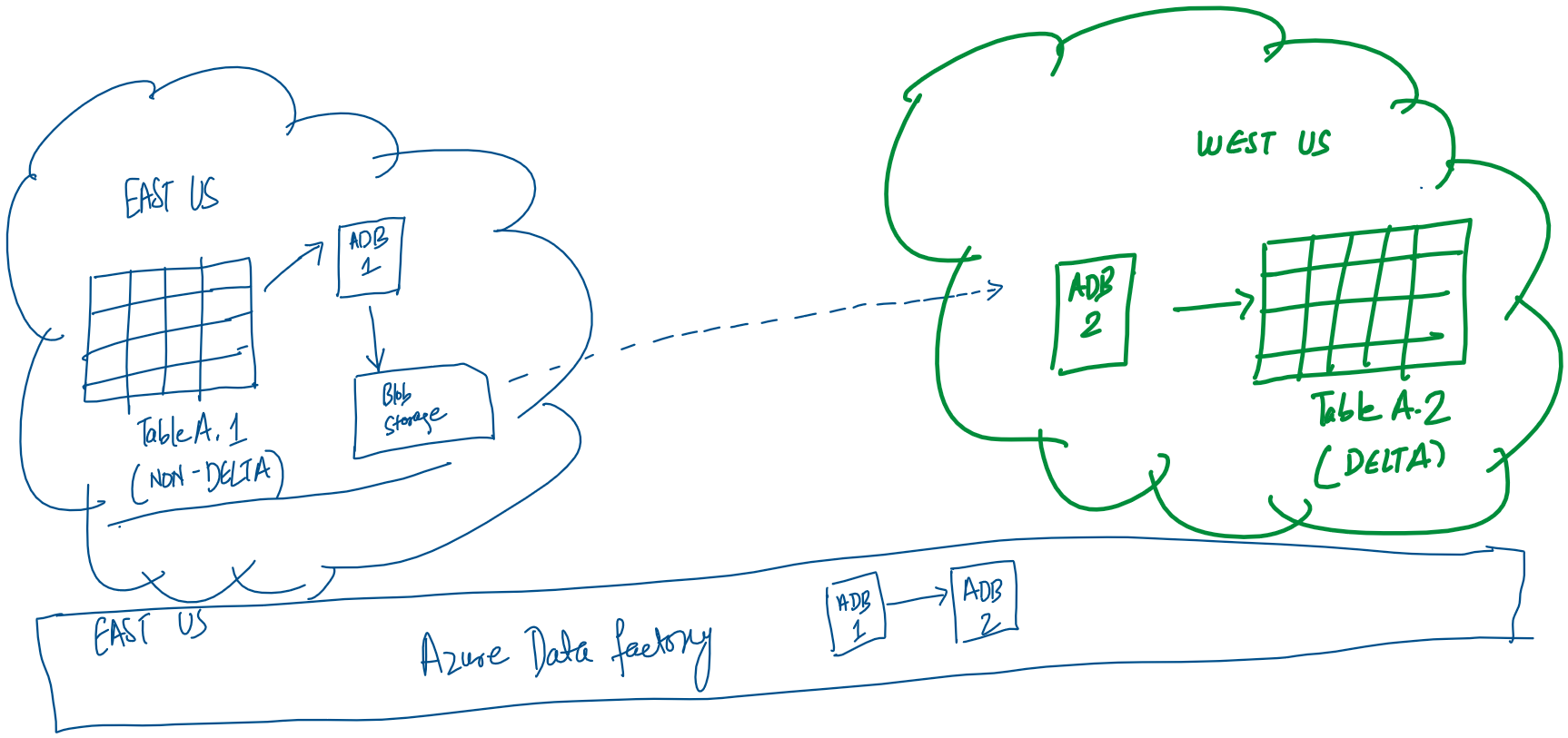
This would be the simplest as we would simply need a Copy Data activity in the pipeline with two linked services. The source would be a Delta Lake linked service to eastus tables and the sink would be another Delta Lake linked service to westus table. This solution faced two practical issues:

  1. The source table was not a Delta table. This prevented the use of Delta Lake linked service as source.
  2. When sink for copy activity is a not a blob or ADLS, it requires us to use a staging storage blob. While we were able to link a staging storage blob, the connection could not be established due to authentication errors during execution. The pipeline error looked like the following:
Operation on target moveBlobToADB failed: ErrorCode=AzureDatabricksCommandError,Hit an error when running the command in Azure Databricks. Error details: shaded.databricks.org.apache.hadoop.fs.azure.AzureException: shaded.databricks.org.apache.hadoop.fs.azure.AzureException: Unable to access container adf-staging in account xxx.blob.core.windows.net using anonymous credentials, and no credentials found for them in the configuration. Caused by: shaded.databricks.org.apache.hadoop.fs.azure.AzureException: Unable to access container adf-staging in account xxx.blob.core.windows.net using anonymous credentials, and no credentials found for them in the configuration. Caused by: hadoop_azure_shaded.com.microsoft.azure.storage.StorageException: Public access is not permitted on this storage account..

On digging deeper, this requirement is documented as a prerequisite. We wanted to use the Access Key method but it requires the keys to be added into Azure Databricks cluster configuration. We didn’t have access to modify the ADB cluster configuration.

To work with this, we found the following alternatives:

  1. Use Databricks notebook to read data from non-Delta Tables in Databricks. The data can be stored in a staging Blob Storage.
  2. To upload the data into the destination table, we will again need to use a Databricks notebook as we are not able to modify the cluster configuration.

Here is the solution we came up with:

In this architecture, the ADB 1 notebook is reading data from Databricks Table A.1 and storing it in the staging blob storage in the parquet format. Only specific users are allowed to access eastus data tables, so the notebook has to be run in their account. The linked service configuration of the Azure Databricks notebook requires us to manually specify: workspace URL, cluster ID and personal access token. All the data transfer is in the same region so no bandwidth charges accrue.

Next the Databricks ADB 2 notebook is accesses the parquet file in the blob storage and loads the data in the Databricks Delta Table A.2.

The above sequence is managed by the Azure Data Factory and we are using Run ID as filenames (declared as parameters) on the storage account. This pipeline is configured to be run daily.

The daily run of the pipeline would lead to a lot of data in the Azure Storage blob as we don’t have any step that cleans up the staging files. We have used the Azure Storage Blob lifecycle management to delete all files not modified for 15 days to be deleted automatically.

Testing SOAP APIs with Telerik Test Studio

The legacy SOAP based web services/ APIs are still in use at a lot of organisations. While Telerik Test Studio has direct support for REST based APIs, testing SOAP web services requires a few additional steps.

In the short video below, we share how we can test SOAP based APIs in Test Studio:

The three things needed include:

  1. A Test Oracle to encapsulate web services call: Built easily with Visual Studio
  2. Coded Steps in Test Studio
  3. Data Driven tests for testing various inputs

The transcript of the video is as follows:

Can Test studio test APIs? And i think most of you know the answer that it does support testing REST APIs. Recently one of the customers asked me if Telerik Test Studio can be used for automation of SOAP-based web services and the answer to that is it can be done in telerik test studio using coded tests.

In this video we will see how we can test SOAP based web services using Test Studio. The soap web service that i am using for testing is a publicly available service that converts digits to numbers. So in this web service i’m going to use the number and what it allows me to do is enter a number so let’s enter 789 and by invoking this i get the the words or the digits converted into words as seven eighty nine. So this is the web service that i’m going to test back in the test studio.

I have authored a test that will feed in various digits and verify if the web service returns the correct words for those digits. For the same i have put in some local data with digits in one column and in words in the second column. So this is going to be a data driven test. Let’s test this with our script. I’m just starting the test with the headless chrome as execution engine because web services don’t have a UI. The test has started and you can see that i’ve got the debugger going and already the test has finished.

Now there were four iterations of this test, this being a data driven test and if you want to see the logs for each of the iterations that’s visible here as well. In iteration number one you will notice the overall result is pass. In fact here it shows we’re using chrome headless version and our test was successful in iteration number two where we had put in two three eight nine the result is fail and the failure information is also mentioned here. Well we were expecting the web service to return two hundred and eighty nine but the web service actually returned two thousand three hundred and eight nine not eighty nine. So this actually indicates a failure on the assertion. Well the test continued because we have marked this step as continue on failure. Iteration number three has result as pass wherein we passed in a single digit 4 and we also got back the same value which is four. Iteration or the last iteration here is checking for digits 10 and inwords it should also be ten and once again the overall result is pass. So here you can see its result is pass but your overall result is a fail because one of the iterations here did actually fail.

So in the next few minutes we will see how we had created this SOAP test in telerik test studio. So to work the magic of a soap api test and it’s actually quite painless in telerik test studio. You need three things:

1. the first is a test oracle number

2. two is the coded step in test studio and

3. number three is data driving the verification

Okay let’s start with the test oracle. The test oracle is an external assembly that you are going to use within test studio inside your script but this assembly is going to be created by someone else. So what i had gotten done was to call the SOAP API using a visual studio function of adding web service reference and created that project as an assembly. Now the next step would be to add that assembly in test studio so if you go to your project and go to settings you will have a section that says script. Now within this section you will notice some assemblies that are automatically referenced here. Now if you notice this reference, this is something that has been added as a custom reference and this is where my test oracle has been created. So this assembly uses a simple function to invoke the SOAP API and provides a simple programmatic interface to invoke this soap service. So if you want to add more test oracles or external assemblies you can click on add reference and that’s what allows you to refer any .NET based assembly. So that takes care of the first step which is of getting a test article in place.

The second step is to add a coded step in my test script so you can add a coded step in test studio by using the step builder. Here where i’ve selected the common and within it there is a coded step and i can click on add step button. And this will add a coded step so that’s already done here. As you can see the coded step i am using is titled sample soap underscore coded step. In fact the code for this is available in the cs file located here. I just opened up the cs file the first thing that i need to do is to add a reference or to soap call namespace now in my function which is called as sample code underscore coded step. I am creating an instance of the object and within this i am passing in the specific digits. And finally i’m asserting if the digit that i have passed is the same as the one it should be in words.

Now the syntax here is slightly different. The syntax looks different because we are actually doing the third step in this demo which is data driving the verification. To data drive the verification as well as input values you’ve got to use the data and the specific column that you have created. So that’s what i’m using, so data and digits. And since the function towords requires me to give in an integer value i’m passing that in to the towords function of the test oracle. So conversion service and the function towords are actually coming from the test oracle. Finally i’m adding an assertion to see if the value that has been returned which is the nword value here and then the value that is there in my data driven column which is called inwords is also mentioned here. So both of them need to match up for this test to succeed. To quickly check where we had put in this data driven values we can go back to the test script and down below next to the test steps you will find the local data tab. And that’s where we can manually add these values.

This demonstration has showed you that Test Studio can be easily used to data drive SOAP based APIs automation

Enjoy watching the video and share your questions in the comments section below.

GTM Catalyst to Offer JetBrains Solutions to Enterprises in India

The development landscape is very heterogenous with multiple teams using different languages. Consequently, development teams need a myraid of solutions that support these languages and tools to accelerate the development.

Today we announce that we are partnering with JetBrains, a leading provider of development, deployment, and collaboration tools (a portfolio of 28 products). With it, GTM Catalyst Private Limited will offer local expertise and support to businesses leveraging JetBrains solutions and will also make them available for purchase in Indian Rupees.

As a JetBrains reseller channel partner, GTM Catalyst Private Limited now offers award-winning developer tools including:


1. IDE: IntelliJ IDEA, PyCharm, WebStorm, RubyMine, GoLand, AppCode, and PhpStorm.
2. Collaboration: Developers benefit from CI/CD tool TeamCity and Spaces.
3. Productivity extensions (.NET): ReSharper, dotTrace, and dotMemory.

The flagship product from JetBrains is IntelliJ IDEA, which maximizes Java developer productivity with its intelligent coding assistance and ergonomic design.

JetBrains IDE for professional developers, PyCharm can help developers using Python, the fastest growing language. For DevOps, CI/CD is supported via TeamCity which is a build management and continuous integration server from JetBrains.

Space, the recently launched all-in-one collaboration solution, provides a toolset for instant communication, software development, and team and project management.

“As a company, JetBrains has strived to make the strongest and most effective tools for software developers and teams. We are committed to supporting developers in India with our wide range of tools. We’re very happy to welcome GTM Catalyst Private Limited as our channel partner in India”, said Javed Mohamed, Regional Head – South Asia at JetBrains.

Read the press release here

Connect Telerik Reporting with Postgres SQL

One of our customers required their Telerik Reporting application to connect with their Postgres SQL (for effect, no not Microsoft SQL Server but the open source Postgres SQL).

While at the outset it may appear to be almost impossible but this task is very easy to implement with Telerik Reporting.

We accomplish this with using ADO.NET driver for Postgres SQL. The same approach can be used for other databases like MySQL.

In this post, we will discuss how to get Telerik Reporting working on .NET Core 3.1.

The first thing is to understand that Telerik Reporting is a framework that has three distinct and independent pieces:

  1. Telerik Report Definition
  2. Telerik Reporting Host Application
  3. Telerik Report Viewer

First you would want to create the Telerik Report Definition (a trdp file). To create this, we use the Telerik Reporting Designer. By default, there is nothing that supports Postgres SQL in there. So, here is the first step – Download the NgpSql driver (the MSI installer).

Once done, this will add a new datasource to the SQL Data Source of the designer:

Click on the SQL Data Source, and add a new data connection. In the dropdown, please select the new available provider “Ngpsql Data Provider”:

Following this you will need to provide the connection string. The Postgres connection string is of the following format:

Host=<server name>;Database=<db name>;Username=<username>;Password=<password>

Provide the relevant SQL statement and complete creating the data connection. The rest of the remaining steps are the same as creating a regular Telerik Report definition.

Make sure that the data is as preview in the report.

The second step, is to configure the hosting application. Since we are now working with .NET core, you can start with the .NET Core WebAPI application template and add relevant nuget packages to the same. Detailed instructions are available here: https://docs.telerik.com/reporting/telerik-reporting-rest-service-aspnetcore-mvc-core3

This will make the host application provide the Telerik Reporting Service. You can check if this the reporting has been correctly setup by browsing to the URL: http://localhost/api/reports/formats

The extra step in the host application is to include an additional nuget package in the host application: Ngpsql

The next change in the host application is changing the connection string and its provider. Specify your connection string in the appSettings.json as follows:

Pay special attention to the providerName above.

Congratulations you are done!!

The third and final piece, the Telerik Report Viewer doesn’t require any changes.

Your host application (in my case a simple HTML 5 application) can now simply render the report from the host application.

References:

https://docs.telerik.com/reporting/knowledge-base/configuring-postgres-with-npgsql

https://www.telerik.com/forums/configure-standalone-report-designer-for-postgresql-data-source

https://docs.microsoft.com/en-us/aspnet/core/security/cors?view=aspnetcore-5.0#enable-cors

How to Download Telerik Software

Login to your account at Telerik.com

There are two ways to download Telerik products, doing so online as laid out in the instructions below or using the Control Panel, which is available for download from your account home page.

Once logged into your account, click the “Products & Subscriptions” button (Please note, the account in the screenshot is a test account, you may have different products listed other than DevCraft Complete)

Next, click on the appropriate product

On the next screen, choose the blue “Download Installer and other resources” button

Click on the product that you wish to install

On the next page, choose to either download the product or the latest internal build of the product. Please make ensure that the License type is “Purchase” and not “Trial”

Webinar: Starting out with aPaaS

Telerik has been at forefront of providing tools for improving developer experiences. Now, a new kind of technology is on the horizon called as aPaaS – Application Platform as a Service.

This technology enables enterprises to create better, cheaper and faster applications with very little code. This is going to be a big boost of developers who are constantly required to deliver top quality code in minimal time. This single technology can enable building visually immersive experiences across web, iOS and Android and engaging chatbots. Not just that, it provides full control over the application code and development experience for developers.

This platform is called Progress Kinvey Studio. In this webinar we will introduce what is aPaaS and Kinvey.

The webinar details are as follows:

When: Thursday, Sept 19 2019, 15:00 – 16:00 hrs (IST)

Register here: https://www.techgig.com/webinar/Beginning-aPaaS-Low-Code-Development-for-Web-Mobile-and-Chat-in-the-Real-World-1608

Presenter: Mr. Abhishek Kant, CEO, GTM Catalyst Pvt Ltd

Who should attend: Project Managers, Developers and CTOs

In the webinar Mr. Abhishek will go over:

*Understand aPaaS concepts
*Visual designer for building apps in a matter of minutes
*Write custom logic and UI to finetune the digital experience
*Round-trip code editing (legible code, and editing in your tool of choice) Code portability (no vendor lock-in)
*Enterprise data and authentication integration (use existing data sources)
*Access to cutting-edge features like Augmented Reality and Chatbots
*Simultaneous web, iOS, and Android development

In the Telerik tradition, we will be giving out 3 T-Shirts to top engaged participants at the webinar.

See you at the webinar!

Code-less way to authenticate to Azure Resource Manager API from Azure App Services

This is a guest post by Sujay Sarma:

Typical examples that show you how to connect from a web application to Azure Resource Manager API have you wading through configuring and meddling with OAuth and Owin, not to mention getting you confused between ADAL, MSAL and the different types of Active Directory tenants offered by Azure. We do not need ANY of that, especially if your web application is going to live on as an Azure App Service.

Teeth gnashing? Mouth Salivating?

dreamstime_xl_43928193The short answer is to use “Azure App Service Authentication”. And it is nothing new. It has been around since at least November 2014 (wow! a little over four years since!). At least for me, though I have seen it plenty of times while configuring my App Services in Azure, I have scarcely looked at what it can do. Until now.

A project I was working on for a client required authenticating Azure subscribers to the portal. Initially, I went with the regular walkthroughs. I went into my Azure Active Directory blade and under App Registrations, created a new app, secrets and so on. But I faced really strange issues: There were no issues for me (developer never faces issues and has zero bugs on their dev box, yeah?). But my client contact could not login. He was using a Hotmail login address. I had to add him as a Guest User in my Active Directory tenant! That was not going to be a viable action plan for any further step of the project.

The problem, I determined, was that folks on my tenant could log in, but not others. Strangely, another friend was able to login — his account was a custom domain hosted within another Azure Active Directory Tenant (he was using his Organization ID and apparently they were Azure subscribers as well).

So, I tried to use Azure B2C. This is an poorly documented system, where the current documentation and the portal’s user experience are so different. Not only that, there is a lot of confusing terminology used in the documents — and you have to register “apps” in at least three places, not to mention the Web App I was trying to configure! Short story: It was a mess!!!

I told everybody I was giving up on the issue. We would find some “manual” way to get people to authenticate. That was when, an unrelated Google search threw up the page on App Service Authentication. I sent the URL to my mobile to read it during dinner and turned off my computer for the day. Even after I had read the article in question, I only thought of writing a small POC to see what it could do. The next morning, I sat down to set it up. And boy, oh boy! was I in for a pleasant surprise!

To save people the trouble of having go through the same trial and error I did, here is a concise walkthrough of how to do it. I must thank Chris Gillum, whose 2016 blog post clued me into the right course correction to get everything working.

The Walkthrough

  1. Log in to the Azure Portal.
  2. If it is already on the menu on your left/right hand-side, use that. Otherwise, click “All Services” and search there. Go into Azure Active Directory”. If you’re having a hard time chasing it down, click here to go there directly (you maybe prompted to login).
  3. Now click on the “App registrations (Preview)” item. The official documentation follows the flow of going into the other “App registrations” — do not do that, that will end up giving you “OAuth v1.0” tokens. We need “OAuth v2.0” tokens. I found this out by trial and error. Click here to go to the right blade.
  4. Open a Notepad window.
  5. Along the top of the applications view, find the button that says “Endpoints” and click that. Towards the bottom of the pane full of URLs, find the one that says “WS-Federation sign-on endpoint” (third from the bottom at this time). Copy that FULL address and paste it into your Notepad. Now, in Notepad, carefully delete the “/wsfed” from the end of that address — be careful not to delete anything before the “/”. To be safe, you can hit CTRL+H, in Find, type “/wsfed”, leave Replace as blank and hit “Replace All”.
  6. Now hit “+ New Registration”. Enter any name. Be aware that what you enter here will be shown in big bold letters when Azure later asks the user trying to login for consent (the “…. is asking you for permission to access…” UI). Select the option “Accounts in any organizational directory”. Leave the “Redirect URI” blank for now, we will come back to it later. Click on Register.
  7. Once the Azure Portal tells you that the application was deployed successfully, find it again in the same “App Registrations (Preview)” screen and click on it to enter it.
  8. From the overview page, find the “Application (client) ID”. It will be a Guid. Hover on the value to make the “copy” icon appear. Click it to copy it.
  9. Switch to your Notepad window, type in “App ID”, hit ENTER and paste what you copied on step 7.
  10. OPTIONAL. Back on the Azure Portal, go into “Branding” and upload a logo. a picture of size 48×48 pixels works best. Anything else will cause the consent screen to appear in strange shapes and sizes. What you enter into the various URL fields there is not relevant — they will be used to show information links at the bottom of the consent screen. You may leave them blank or enter valid URLs into them — they need not even be on your website!
  11. IMPORTANT. Go into “Certificates & Secrets”. Under the “Client secrets” heading, click “+ New client secret”. Enter a name (does not matter, it is for your convenience), select an expiry value (“Never” is all you need). Click Add. When the new password is generated, it will be shown there. Again, hover on the value under the “VALUE” heading to make the little icon appear and copy it (if you don’t copy it fully, you will be in a world of pain).
  12. Switch to your Notepad window, type in “Secret”, hit ENTER and paste what you copied in step 10.
  13. IMPORTANT. Go into “API Permissions”. Click on “+ Add a permission”. Select “Microsoft Graph” (at the time of writing this, it is a large banner like button right on top of the list that appears). Select “Delegated Permissions”. Check ON: email, offline_access, openid and profile. Scroll to the bottom and find “User”, expand it and check ON “User.Read”. Click “Add permissions” at the bottom.
  14. Now click the “+ Add a permission” again. This time, select “Azure Service Management” (there are many similar looking “Azure” permissions on the list, select the right one). There is only one permission at this time, select it (or select “user_impersonation” if you find more permissions when you’re reading this!). Click “Add permissions” at the bottom.
  15. Right-click on the “App Services” menu item on the navigation (or find it under “All Services”) and select to open it in a new tab — you need to come back to the settings you were working with so far — we are not done there yet! Anyway, end up here.
  16. NOTE: If you already have an app service that you are configuring this for, you can use that. Otherwise, create a new app service. There is nothing special to be done there — and you don’t need to upload any code YET. Once you have selected the app service or created one, continue below.
  17. Select the App Service, open its Authentication/Authorization blade. Set the “App Service Authentication” option to “On”. Immediately a bunch of options will appear below it.
  18. We are only interested in the “Azure Active Directory” option in this walkthrough. So select that. A new blade will open.
  19. Select “Advanced”. A different set of options will appear under it.
  20. For “Client ID”, paste the value pasted under “App ID” from your Notepad window.
  21. Under “Issuer Url” paste the URL you pasted from Step 5 above (it will look like “https://login.microsoftonline.com/…&#8221;).
  22. Under “Client Secret”, paste in the value under “Secret” from your Notepad window.
  23. Now, this is very important. Under “Allowed Token Audiences”, first paste in “https://management.core.windows.net/&#8221;, tab out. Another text box will appear. Now paste in “https://management.azure.com/&#8221; (ensure the final “/” are there). This tells the system to get you the Bearer Tokens that will work with the Azure REST API 🙂 This is the secret magic sauce to the whole thing!
  24. Click OK.
  25. Back on the “Authentication / Authorization” blade, select one of “Allow Anonymous requests (no action)” or “Login with Azure Active Directory”. If you plan to show a “Sign in” link on your website — that is, you want the user to see something before they need to login, then use the “Allow Anonymous requests (no action)” option. If like with the Azure Portal, you want them to be signed in from the get-go, use the “Login with Azure Active Directory” option.
  26. Ensure “Token Store” (bottom of the page, under “Advanced settings”) is “On”.
  27. Click “Save” on top of the page to save everything.
  28. IMPORTANT CAVEAT: If at any point of time, you make changes to this set up, you will need to Restart your App Service before it will use the new values.
  29. Go into the “Overview” blade of your App Service. Wait for all the properties on the top panel to load, and copy the full value of the “URL” (“https://xyz.azurewebsites.net&#8221;). Note how this is “https” ?
  30. Now go back to the Azure Directory screen — if you left it open in another tab or window at the end of step 14, switch to that tab. Otherwise, navigate to it from the menu, or click here.
  31. Ensure you are within the Azure Directory Application (the one you configured from step 3 to 14).
  32. Click into the “Authentication” tab.
  33. Under “Redirect URIs”, ensure “Web” is selected for “TYPE”, under “REDIRECT URI”, paste in the URL to the App Service (Step 29). At the end of this URL, paste in “/.auth/login/aad/callback” [be careful to paste in everything between the quotes]. Note that there is a dot (“.”) in front of “auth”. Your final URL should look like: “https://contoso.azurewebsites.net/.auth/login/aad/callback“.
  34. Scrolling down, under Advanced settings, paste/enter the Logout URL to make it thus: “https://contoso.azurewebsites.net/.auth/logout“. Again, note the “.” in front of “auth”.
  35. Scrolling down, under “Implicit grant”, check ON both “Access tokens” and “ID tokens”.
  36. Click Save above.

Your Azure configuration is DONE.

From your App Service Code

Fire up Visual Studio, create a new web application. I am using a regular Web Forms application. You are free to do this in MVC or .NET Core or whatever. I am using Visual Studio 2019, and selected the “ASP.NET Web Application (.NET Framework)” option. If you are prompted to select the type of authentication — leave it as “No authentication”.

You do not need to install new NuGet packages! Azure App Service automatically fetches the right Bearer token for you (without any plumbing!). This is available to you in the Request Header “X-MS-TOKEN-AAD-ACCESS-TOKEN”. Fetch it from:

string token = Request.Headers[“X-MS-TOKEN-AAD-ACCESS-TOKEN”];

You can now pass this token to your AzureRM REST API calls. I do not use any of the Azure SDKs to talk to AzureRM, and write System.Net.HttpClient based GET/PUT/etc calls. My code to pull all the subscriptions for a logged in user now looks like this:

HttpRequestMessage request = new HttpRequestMessage(HttpMethod.Get, “https://management.azure.com/subscriptions?api-version=2019-03-01&#8221;);

request.Headers.Authorization = new AuthorizationHeaderValue(“Bearer”, Request.Headers[“X-MS-TOKEN-AAD-ACCESS-TOKEN”]);

HttpResponseMessage response = await client.SendAsync(request);

Simple, huh?

The “Post Digital” Enterprise

choiceDigital Transformation has graduated from being a differentiating advantage to now being the price of admission. Enterprises must now use the data and experiences collected in the earlier phase and use powerful new technologies to innovate in their business models and personalize experiences for their customers.

According to a recently released Accenture Technology Vision 2019 report, nearly four in five (79 percent) of more than 6,600 business and IT executives worldwide  surveyed believe that digital technologies ― specifically social, mobile, analytics and cloud ― have moved beyond adoption silos to become part of the core technology foundation for their organization. Respondents were C-level executives and directors at companies across 27 countries and 20 industries, with the majority having annual revenues greater than US$6 billion.

5 technology trends identified in the report, that can provide the elusive competitive edge to the willing enterprise are as follows:

  1. DARQ Power: This newly coined phrase stands for distributed ledgers, artificial intelligence, extended reality and quantum computing (DARQ). Amongst these 41 percent of executives ranked AI as number one in terms of impact.
  2. Unlock new opportunities: Leverage data captured from interactions to deliver rich, individualized, experience-based relationships. More than four in five executives (83 percent) said that digital demographics give their organizations a new way to identify market opportunities for unmet customer needs.
  3. Human+ Worker: The typical employee is digitally savvy with two-thirds (71 percent) of executives believe that their employees are more digitally mature than their organization, resulting in a workforce “waiting” for the organization to catch up.
  4. Security Flow: Security is no more limited to enterprise boundaries. The interconnectedness between these connections increase companies’ exposures to risks. Only 29 percent of executives said they know their ecosystem partners are working diligently to be compliant and resilient with regard to security.
  5. Meet consumers at the speed of now: Direct digital access to customers and powerful analytics capabilities enable innovative personalization strategies. Six in seven executives (85 percent) said that the integration of customization and real-time delivery is the next big wave of competitive advantage.

The focus on personalisation as a differentiator is foremost in the report. I had highlighted a similar trend in an interview with Marketing with Maveriks podcast in Jan 2019.

From my universe, Sitefinity is a wonderful digital marketing tool that provides for static and dynamic personalisation across channels.

Have thoughts around where we are headed? Leave a comment below..

Awarded 10 Most Promising Machine Learning Solution Providers

We are pleased to share that GTM Catalyst has been awarded as “10 Most Promising Machine Learning Solution Providers” in India by CIOReview.CIOReviewMostPromising

Here is a brief introduction of the award by CIOReview Magazine:

CIOReview India presents a list of “10 Most Promising Machine Learning Solution Providers”. Being closely scrutinized by a distinct panel of judges including CEOs, CIOs, CXO, analysts and CIOReview editorial board, we believe these solution vendors can bridge the gap between businesses and solution providers that are transforming business processes through their significant offerings.

Few extracts from the feature:

The top use case for AI has been customer facing technologies like conversation chatbots. Acknowledging these needs Gurgaon headquartered GTM Catalyst provides customer facing AI solutions notably the conversational chatbots under the KatalystAI platform that have been utilized by industries such as medical institutions, consumer electronics,
and automobiles sector.

KatalystAI platform is a System of Intelligence for enterprises.

The KatalystAI platform of GTM Catalyst serves to augment the robust sales forecasting processes that exist within an organization by employing the latest Machine Learning algorithms like boosted decision trees and deep learning algorithms.

The entire feature can be downloaded from here.

How-To: Create Charts with Kendo UI with Remote Data

If you know jQuery, and want to include data vizualization elements in your web page without all the hassle, you are at the right place. In this post, we are going to give you a quick view of how Kendo works with jQuery to create a pie chart.

We will build a ratings pie chart, step by step. Final product is shown below.

1. API

We need access to an API which we can call to get our remote data in the form of json. An API like this:

https://<some-url>/totalratings

which gives data in the form of json like this:

[
  {
    category: "Asia",
    value: 53.8,
    color: "#9de219"
  },
  {
    category: "Europe",
    value: 16.1,
    color: "#90cc38"
  },
  {
    category: "Latin America",
    value: 11.3,
    color: "#068c35"
  },
  {
    category: "Africa",
    value: 9.6,
    color: "#006634"
  },
  {
    category: "Middle East",
    value: 5.2,
    color: "#004d38"
  },
  {
    category: "North America",
    value: 3.6,
    color: "#033939"
  }
]

should do the work. The data must be a json or an array of json.

Note: If you’re the developer of the API, then make sure to modify the json to make it compatible with Kendo before sending it as response. Check out Kendo demos for more info.

2. Download

Now you need to download Kendo UI. There are several paid versions, and a free (trial) version. Trial is more than enough for trying it out.

Download Kendo UI for a trial period from here. You will have to sign up to download it.

3. Transport

Extract the downloaded ZIP archive to an easily accessible location. We are going to need it’s js and css folders.

4. Kickstart

Kickstart the project by creating a new folder, say kendo-pie. Copy the downloaded js and css folders in kendo-pie.

Now, create a new HTML file in kendo-pie, say index.html. This is our main webpage. The pie chart will reside here.

5. The HTML

Open index.html with your favourite text editor. Add some starter code.

Give it a title, say Overall Ratings. Link all the necessary js and css files, inside head.

Time to populate the body. Create a wrapper (div), with id overall. The actual chart element and it’s script will reside in this wrapper. Create the chart div inside the wrapper, with id chart. Give it some style with a style attribute.

The above goes inside body, and the whole thing up-to this point looks something like this:

6. The jQuery

Create a script element inside the wrapper, and add some starter jQuery code.

Inside the document-ready function, select the chart element with jQuery’s id selector, and apply kendoChart() method.

7. The Kendo

kendoChart() takes a configuration object as an argument. This configuration object is used to describe the chart and include data (local or remote) to be represented.

Let’s contsruct the configuration object:

  1. Add title property.

2. Add dataSource property: read and dataType.

3. Add seriesDefaults property.

4. Add series property: field and categoryField.

5. Add tooltip property.

kendoChart() method is ready. So is the script. Coding part is complete.

These were the basic steps to create a pie chart using jQuery and Kendo, mostly Kendo. Now, open index.html in browser, and you should see output as below.

I hope the above steps were helpful in giving you a basic idea about Kendo UI. It’s up to you now to tweak the chart however you want, or create a new element altogether.

Documentation on the customization options are available here, and demos here.

Authored by: Abhay Kumar.