We recently had a case where a customer was running Azure Databricks notebook from Azure Data Factory. They mentioned that the configuration used to run the notebook was not secure as it was associated with a user account (probably a service account). The username and password was known to multitude of users and it had already caused some trouble. The concept of a “service account” has been quite prevalent since the times of on-premise applications. The service account was a user account that was used to run various applications and nothing else. In the modern world of cloud services, service accounts are obsolete and should never be used.
He wondered if there was a better way to run such notebooks in a more secure way?
In a single line, the solution to this problem is running the notebook as a service principal (and not a service account).
Here is a detailed step by step guide on how to make this work for Azure Databricks notebooks running from Azure Data Factory:
- Generate a new Service Principal (SP) in Azure Entra ID and create a client secret
- Add this Service Principal to the Databricks workspace and grant “Cluster Creation” rights
- Grant this Service Principal User Access to the Databricks workspace as a user
- Generate a Databricks PAT for this Service Principal
- Create a new Linked Service in ADF using Access Token credentials of the Service Principal
- Create a new workflow and execute it
If you followed the above instructions, your Databricks notebook will be run as a Service Principal.
One thing to understand before going over the detailed steps is the fact that when you add a Databricks notebook as an activity in Azure Data Factory, you are creating an “ephemeral job” in Databricks in the background when the ADF pipeline is run. You can control what kind of job cluster gets created and the user credentials under which the job will be run based on the linked service settings. Let’s get started:
- Generate a new SP with client secret
- Go to portal.azure.com and search for “Microsoft Entra ID” in the search tab and click it
- Click on Add and select “App registration”
- Give a meaningful name and leave the rest as-is and click “register”
- You should now see something like below
- Now click on “Certificates & secrets” and under the “Client secrets” tab click “New client secret”
- Under the “Add a client secret” pop-up, give a meaningful description and choose the appropriate expiration window and click “create”. Once done you should see something like this under the “Client secrets” tab
- Now open a notepad and have all the information noted there.
Host: Databricks workspace URL
Azure_tenant_id and Azure_client_id will be what is shown in the image under point 4
Azure_client_secret will be the value in the image under point 6


2. Add this Service Principal to the Databricks workspace and grant “Cluster Creation” rights
- Now go to your target workspace and click on your Name to expand the menu, click open the settings( this requires workspace admin privilege)
- Now click on” identity and access” and under service principals click on manage


Click on “add service principal” button
Now click on Add new
Select the “Microsoft Entra ID managed” radio button and populate with the Application ID(client id) and give the same name as shown in point 4 and click Add
Now provide “Allow cluster creation” permission to the service principal to ensure it can create a new job cluster when we run through an ADF and click “update”


Generate a Databricks PAT for this Service Principal
- If you are on Mac open the terminal and use the command “nano .databrickscfg” to open the databricks config file and paste the information from the notepad from point 8.
If you are on Windows press windows + R and type “notepad
%APPDATA%\databricks\databricks.cfg” and press enter. Now paste the information from the notepad from point 8 into the Databricks config file. You will also have to give a meaningful profile name to identify the workspace in the config file.
The config file should look like below once you are done. [hdfc-dbx] is the profile name here.Save and exit.
- Now go to Databricks CLI and authenticate the service principal’s profile using a PAT token by typing “databricks configure”. It will prompt for the host workspace’s URL and PAT token, provide it, and press enter.
- Now goto databricks cli and generate a PAT token for the Service Principal using the command “databricks tokens create –lifetime-seconds 86400 -p <profile name>”. You should see a proper response like below:
- Now grab the “token value” and keep it in a notepad safely

Create a new Linked Service in ADF using Access Token credentials of the Service Principal
- Now go to ADF, click on Manage -> Linked services -> New
Under New Linked Service popup click on “compute” and select “Azure Databricks” click continue - Now provide a meaningful name to the linked service, select the proper Azure subscription, and your target workspace. Under Authentication Type leave the option as Access Token and under the access token field update the access token we generated in point 13.(This is being done as an interim solution, the best practice is to use an Azure Key Vault and pass the token through secret).
- Now select the cluster version as 13.3 LTS, Node type, Python version, and Worker options as relevant to current cluster configuration. You can select the UC Catalog Access Mode as “Assigned” for single user and “Shared” for shared access mode. Click on test connection to ensure everything is working as intended.

Create a new workflow and execute it
- Now create a pipeline select the linked service that you created and point the ADF to a notebook.
- Click “Debug” and the job should run successfully


If you open the job execution link, you can see the job has been run as a Service Principal under task details

This is indicated by the value against “Run as” which is that of the Service Principal.


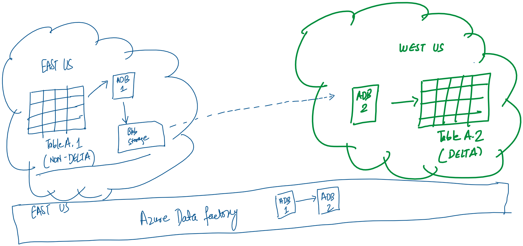
 This would be the simplest as we would simply need a Copy Data activity in the pipeline with two linked services. The source would be a Delta Lake linked service to eastus tables and the sink would be another Delta Lake linked service to westus table. This solution faced two practical issues: