Introduction to Machine Learning with Spark ML – III

In the last post, we saw how we can use Pipelines to streamline our machine learning workflow.

We will start off with a fantastic feature that will blow the lid off your mind. All the effort done till now, in post I and II, can be done in 2 lines of code! Ah yes, this magic is possible with use of a feature called AutoML. Not only will it perform preprocessing steps automatically, it will also select the best algorithm from a multitude of them including XGBoost, LightGBM, Prophet etc. The hyper parameter search comes for free 🙂 If all this was not enough it will share the entire auto-generated code for your use and modification. So, the two magic lines are:

from databricks import automl
summary = automl.classify(train, target_col="category", timeout_minutes=20)

The AutoML requires you to specify the following:

  1. Type of machine learning problem – Classification/ Regression/ Forecasting
  2. Specify the training set, target column
  3. Timeout after which the autoML will stop looking for better models.

While all this is very exciting, the real world use case of AutoML tends to be to create a baseline for model performance and give us a model to start with. In our case, the AutoML gave an RoC score of 91.8% (actually better than our manual work so far!!) for the best model.

Looking at the auto-generated Python notebook, here are the broad steps it took:
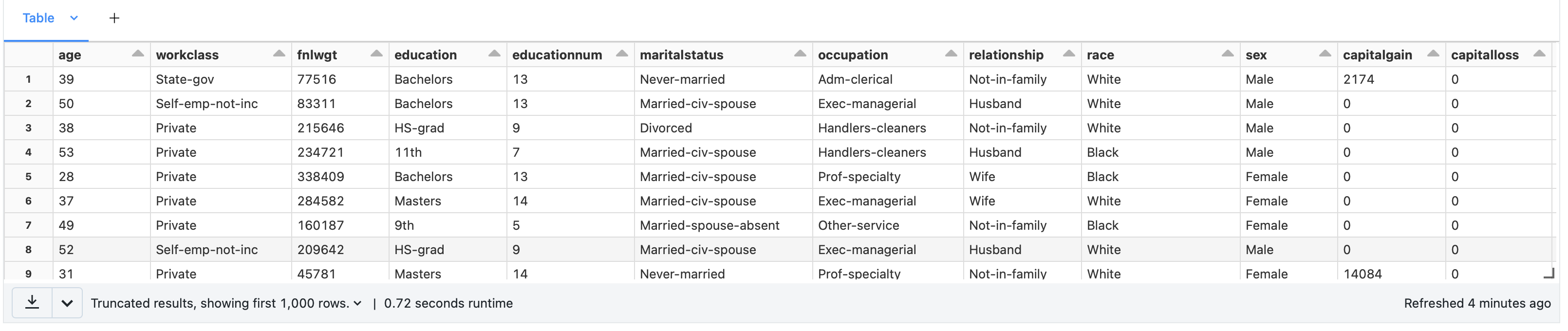
  1. Load Data
  2. Preprocessing
    • Impute values for missing numerical columns
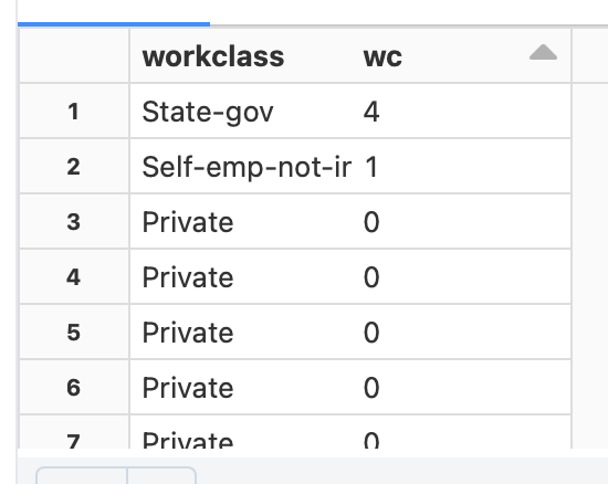
    • Convert each categorical column into multiple binary columns through one-hot encoding
  3. Train – Validation – Test Split
  4. Train classification model
  5. Inference
  6. Determine Accuracy – Confusion matrix, ROC and Precision-Recall curves for validation data

This is broadly in line with what we did in our manual setup.

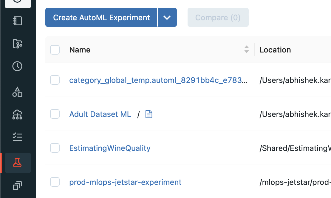
Apart from the coded approach we saw, you can create AutoML experiment using the UI from the Experiments -> Create AutoML Experiment button. If you can’t find the experiments tab, make sure that you have the Machine Learning persona selected in the Databricks workspace.

In an enterprise/ real world scenario, we will build many alternate models with different parameters and use the one with higest accuracy. Next, we deploy the model and use it for predictions with new data. Finally, the selected model will be updated over time as new data becomes available. Until now, we didn’t talk about how to handle these enterprise requirements or were doing it manually on best effort.

These requirements are covered under what we know as MLOps. Spark supports MLOps using an open source framework called MLFlow. MLFlow supports the following objects:

  1. Projects: Provides a mechanism for storing machine learning code in a reusable and reproducible format.
  2. Tracking: Allows for tracking your experiments and metrics. You can see the history of your model and its accuracy evolve over time. There is also a tracking UI available.
  3. Model Registry: Allows for storing various models that you develop in a registry with an UI to explore the same. It also provides for model lineage (which MLflow experiment and run produced the model), stage transitions (for example from staging to production)
  4. Model Serving: We can use serving to provide inference endpoints for either batch or inline processing. Mostly this will be made available as REST endopoints.

There is a very easy way to get started with MLFlow where we allow MLFlow to log automatically the metrics and models. This can be done using a single line:

import mlflow
mlflow.autolog()

This will log the parameters, metrics, models and the environment. The core concept to get with MLOps is the concept of runs. Each run is a unique combination of parameters and algorithm that you have executed. Many runs can be part of the same experiment.

To get started we can set name of the experiment with the command: mlflow_set_experiment(“name_of_the_experiment”)

To start tracking the experiments manually, we can setup the context as follows:

with mlflow.start_run(run_name="") as run:
   <pseudo code for running an experiment>
   mlflow.log_param("key","value")
   mlflow.log_metrics("key","value")
   mlflow.spark.log_model(model,"model name")

You can track parameters and metrics using log_param and log_metrics functions of mlflow object. The model can now be registered with the Model Registry using the function: mlflow.register_model(model_uri=””, name=””)

What is important here is the model_uri. The model_uri takes the form: runs:/<runid>/model. The runid identifies the specific run in the experiment and each model is stored at the model_uri location mentioned above.

You can now load the model and perform inference using the following code:

import mlflow

# Load model
loaded_model = mlflow.spark.load_model(model_uri)

# Perform inference via model.transform()
loaded_model.transform(data)

While we have seen how to track experiments explicitly, Databricks Workspaces also track the experiments automatically (from Databricks Runtime 10.3 ML and above). You can view the expriments and their runs in the UI via the Experiments sidebar of the Machine Learning persona.

You will need to click on the specific experiment (in our case Adult Dataset), that will show all the runs of the experiment. Click on the specific run to get more details about the run. The run will show the metrics recorded which is in our case was areaUnderRoC of 91.4%.

Under Artifacts, if you click on the model, you can see the URI of the model run. This URI can be used to register the model with the Model Registry and use it for predictions at any point in time.

MLFlow also supports indicating the state of the model for production. Different states supported by MLFlow are:

  1. None
  2. Staging
  3. Production
  4. Archived

Once your model is registered with the Model registry, you can change the state of the model to any other state with the function transition_model_version_stage() function.

From the model registry you are able to create model serving endpoint using the Serverless Real-Time Inference service that uses managed Databricks compute service to provide a REST endpoint.

Introduction to Machine Learning with Spark ML – II

In the earlier post, we went over some concepts regarding Machine Learning done with Spark ML. Here are primarily 2 types of objects relating to machine learning we saw:

  1. Transformers: Objects that took a DataFrame, changed something in it and returned a DataFrame. The method used here was “transform”.
  2. Estimator: Objects that are passed in a DataFrame and would apply an algorithm on it to return a transformer. E.g. GBTClassifier. We used the “fit” function to apply the algorithm on the Dataframe.

In our last example of predicting income level using Adult dataset, we had to change our input dataset to a format that is suitable for machine learning. There was a sequence of changes we had done e.g. converting categorical variables to numeric, One Hot Encoding & Assembling the columns in a single column. Everytime there is additional data available (which will be numerous times), we will need to do these steps again and again.

In this post, we will introduce a new Object that organises these steps in sequence that can be run as many times as needed and it is called the Pipeline. The Pipeline chains together various transformers and estimators in sequence. While we could do the machine learning without the Pipeline, it is a standard practice to put the sequence of steps in a Pipeline. Before we get there, let’s try to add an additional step in fixing our pipeline and that is to identify and remove Null data. This is indicated in our dataset as ‘?’.

To know how many null values exist let’s run this command:

from pyspark.sql.functions import isnull, when, count, col
adultDF.select([count(when(isnull(c), c)).alias(c) for c in adultDF.columns]).show()

The result shows that there are no null values. Inspecting the data, we see that null values have been replaced with “?”. We would need to remove these rows from our dataset. We can replace the ? with null values as follows:

adultDF = adultDF.replace('?', None)

Surprisingly this doesn’t change the ? values. It appeared that the ? is padded with some spaces. So we will use the when and trim function as follows:

from pyspark.sql.functions import isnull, when, count, col,trim
adultDF = adultDF.select([when(trim(col(c))=='?',None).otherwise(col(c)).alias(c) for c in adultDF.columns])

This replaces ? will null that we can now drop from our dataframe using dropna() function. The number of rows remaining are now 30,162.

Now let’s organise these steps in a Pipeline as follows:

from pyspark.ml import Pipeline

adultPipeline = Pipeline(stages = [wcindexer,eduindexer,maritalindexer,occupationindexer,relindexer,raceindexer,sexindexer,nativecountryindexer,categoryindexer,ohencoder,colvectors])

The stages list contains all the transformers we used to convert raw data into dataset ready for machine learning. This includes all the StringIndexers, OneHotEncoder and VectorAssembler. Next, the process of defining the GBTClassifier and BinaryClassificationEvaluator remains the same as in the earlier post. You can now include the GBTClassfier in the pipeline as well and run the fit() on this pipeline with train dataset as follows:

adultMLTrainingPipeline = Pipeline(stages = [adultPipeline,gbtclassifier])
gbmodel  = adultMLTrainingPipeline.fit(train)

However, we can perform another optimization at this point. The model currently trained is based of a random split of values from the dataset. Cross Validation can help generalise the model even better by determining best parameters from a list of parameters and do it by creating more than one train and test datasets (called as folds). The list of parameters are supplied as ParamGrid as follows:

from pyspark.ml.tuning import CrossValidator, ParamGridBuilder

paramGrid = ParamGridBuilder()\
  .addGrid(gbtclassifier.maxDepth, [2, 5])\
  .addGrid(gbtclassifier.maxIter, [10, 100])\
  .build()

# Declare the CrossValidator, which performs the model tuning.
cv = CrossValidator(estimator=gbtclassifier, evaluator=eval, estimatorParamMaps=paramGrid)

The cross validator object takes the estimator, evaluator and the paramGrid objects. The pipeline will need to be modified to use this cross validator instead of the classifier object we used earlier as follows:

adultMLTrainingPipeline = Pipeline(stages = [adultPipeline,gbtclassifier])


adultMLTrainingPipeline = Pipeline(stages = [adultPipeline,cv])

With these settings, the experiment ran for 22 mins and the evalution result came out to be 91.37% area under RoC.

Introduction to Machine Learning with Spark ML – I

Machine Learning is most widely done using Python and scikit-learn toolkit. The biggest disadvantage of using this combination is the single machine limit that Python imposes on training the model. This limits the amount of data that can be used for training to the maximum memory on the computer.

Industrial/ enterprise datasets tend to be in terabytes and hence the need for a parallel processing framework that could handle enormous datasets was felt. This is where Spark comes in. Spark comes with a machine learning framework that can be executed in parallel during training using a framework called Spark ML. Spark ML is based on the same Dataframe API that is widely used within the Spark ecosystem. This requires minimal additional learning for preprocessing of raw data.

In this post, we will cover how to train a model using Spark ML.

In the next post, we will introduce the concept of Spark ML pipelines that allow us to process the data in a defined sequence.

The final post will cover MLOps capabilities that MLFlow framework provides for operationalising our machine learning models.

We are going to be Adult Dataset from UCI Machine Learning Repository. Go ahead and download the dataset from the “Data Folder” link on the page. The file you are interested to download is named “adult.data” and contains the actual data. Since the format of this dataset is CSV, I saved it on my local machine as adult.data.csv. The schema of this dataset is available in another file titled – adult.names. The schema of the dataset is as follows:

age: continuous.
workclass: categorical.
fnlwgt: continuous.
education: categorical.
education-num: continuous.
marital-status: categorical.
race: categorical.
sex: categorical.
capital-gain: continuous.
capital-loss: continuous.
hours-per-week: continuous.
native-country: categorical.
summary: categorical

The prediction task is to determine whether a person makes over 50K in a year which is contained in the summary field. This field contains value of <50K or >=50K and is our target variable. The machine learning task is that of binary classification.

Upload file in DBFS

The first step was to upload the dataset from where it is accessible. I chose DBFS for ease of use and uploaded the file at the following location: /dbfs/FileStore/Abhishek-kant/adult_dataset.csv

Once loaded in DBFS, we need to access the same as a Dataframe. We will apply a schema while reading the data since the data doesn’t come with header values as indicated below:

adultSchema = "age int,workclass string,fnlwgt float,education string,educationnum float,maritalstatus string,occupation string,relationship string,race string,sex string,capitalgain double,capitalloss double,hoursperweek double,nativecountry string,category string"

adultDF = spark.read.csv("/FileStore/Abhishek-kant/adult_dataset.csv", inferSchema = True, header = False, schema = adultSchema)

A sample of the data is shown below:

We need to move towards making this dataset machine learning ready. Spark ML only works with numeric data. We have many text values in the dataframe that will need to be converted to numeric values.

One of the key changes is to convert categorical variables expressed as string into labels expressed as string. This can be done using StringIndexer object (available in pyspark.ml.feature namespace) as illustrated below:
eduindexer = StringIndexer(inputCol=”education”, outputCol =”edu”)

The inputCol indicates the column to be transformed and outputCol is the name of the column that will get added to the dataframe after converting to the categorical label. The result of the StringIndexer is shown to the right e.g. Private is converted to 0 while State-gov is converted to 4.

This conversion will need to be done for every column:

#Convert Categorical variables to numeric
from pyspark.ml.feature import StringIndexer

wcindexer = StringIndexer(inputCol="workclass", outputCol ="wc")
eduindexer = StringIndexer(inputCol="education", outputCol ="edu")
maritalindexer = StringIndexer(inputCol="maritalstatus", outputCol ="marital")
occupationindexer = StringIndexer(inputCol="occupation", outputCol ="occ")
relindexer = StringIndexer(inputCol="relationship", outputCol ="relation")
raceindexer = StringIndexer(inputCol="race", outputCol ="racecolor")
sexindexer = StringIndexer(inputCol="sex", outputCol ="gender")
nativecountryindexer = StringIndexer(inputCol="nativecountry", outputCol ="country")
categoryindexer = StringIndexer(inputCol="category", outputCol ="catlabel")

This creates what is called a “dense” matrix where a single column contains all the values. Further, we will need to convert this to “sparse” matrix where we have multiple columns for each value for a category and for each column we have a 0 or 1. This conversion can be done using the OneHotEncoder object (available in pyspark.ml.feature namespace) as shown below:
ohencoder = OneHotEncoder(inputCols=[“wc”], outputCols=[“v_wc”])

The inputCols is a list of columns that need to be “sparsed” and outputCols is the new column name. The confusion sometimes is around fitting sparse matrix in a single column. OneHotEncoder uses a schema based approach to fit this in a single column as shown to the left.

Note that we will not sparse the target variable i.e. “summary”.

The final step for preparing our data for machine learning is to “vectorise” it. Unlike most machine learning frameworks that take a matrix for training, Spark ML requires all feature columns to be passed in as a single vector of columns. This is achieved using VectorAssembler object (available in pyspark.ml.feature namespace) as shown below:

colvectors = VectorAssembler(inputCols=["age","v_wc","fnlwgt","educationnum","capitalgain","capitalloss","v_edu","v_marital","v_occ","v_relation","v_racecolor","v_gender","v_country","hoursperweek"],
outputCol="features")

As you can see above, we are adding all columns in a vector called as “features”. With this our dataframe is ready for machine learning task.

We will proceed to split the dataframe in training and test data set using randomSplit function of dataframe as shown:

(train, test) = adultMLDF.randomSplit([0.7,0.3])

This will split our dataframe into train and test dataframe in 70:30 ratio.
The classifier used will be Gradient Boosting classifier available as GBTClassifier object and initialised as follows:

from pyspark.ml.classification import GBTClassifier

classifier = GBTClassifier(labelCol="catlabel", featuresCol="features")

The target variable and features vector column is passed as attributes to the object. Once the classifier object is initialised we can use it to train our model using the “fit” method and passing the training dataset as an attribute:

gbmodel = classifier.fit(train)

Once the training is done, you can get predictions on the test dataset using the “transform” method of the model with test dataset passed in as attribute:

adultTestDF = gbmodel.transform(test)

The result of this function is addition of three columns to the dataset as shown below:

A very important task in machine learning is to determine the efficacy of the model. To evaluate how the model performed, we can use the BinaryClassificationEvaluator object as follows:

from pyspark.ml.evaluation import BinaryClassificationEvaluator

eval = BinaryClassificationEvaluator(labelCol = "catlabel", rawPredictionCol="rawPrediction")

eval.evaluate(adultTestDF)

In the initialisation of the BinaryClassificationEvaluator, the labelCol attribute specifies the actual value and rawPredictionCol represents the predicted value stored in the column – rawPrediction. The evaluate function will give the accuracy of the prediction in the test dataset represented as AreaUnderROC metric for classification tasks.

You would definitely want to save the trained model for use later by simply saving the model as follows:

gbmodel.save(path)

You can later retrieve this model using “load” function of the specific classifier:

from pyspark.ml.classification import GBTClassificationModel
classifierModel = GBTClassificationModel.load(path)

You can now use this classification model for inferencing as required.